Estimating Future Stock Market Returns

Butler Philbrick & Associates

By Adam Butler and Mike Philbrick

September 26, 2011

The purpose of this paper is not to make bold predictions about stock market prospects on the basis of a detailed narrative or game theory. While most of us would rather hear a good story about how the future is going to unfold, we endorse the decisive evidence that markets and economies are complex, dynamic

systems which are not reducible to normal cause-effect analysis. That said, history has demonstrated time and again that markets oscillate from very cheap to very expensive over many years. Further, we know that long periods of poor returns follow expensive markets, while long periods of rich returns follow cheap

markets. These relationships can be capture quantitatively with fairly simple statistical models that offer surprisingly accurate forecasts about how the future is likely to unfold. Stories may be entertaining and intellectually compelling, but numbers don’t lie.

With this study we wanted to achieve two important objectives:

1. To discover which measures of stock valuations carry meaningful information about future return

2. To create a multi-factor model using the best indicators to forecast future stock market returns over horizons from 5 to 30 year

Please note that all return forecasts in this study are real, inflation adjusted returns to U.S. stocks in including reinvested dividends. The real return data was sourced from Dr. Robert Shiller’s comprehensive database of historical stock market prices found at http://www.econ.yale.edu/~shiller/data.htm, with important contributions and real-time updates from Col. Chris Turner, who publishes the provocative Forecasting the Market: A Thought Experiment report.

There are several reasons why it may be useful to have a robust estimate of future expected returns on stocks:

People who are approaching retirement need to estimate probable returns in order to budget how much they need to save.

A retiree’s level of sustainable income is largely dictated by expected returns over the early years of retirement.

Investors of all types must make an informed decision about how best to allocate their capital among various investment opportunities

Many studies have attempted to quantify the relationship between  Shiller PE and future stock returns. Shiller PE smoothes away the spikes and troughs in corporate earnings which occur as a result of the business cycle by averaging inflation-adjusted earnings over rolling historical 10-year windows.

This study contributes substantially to research on smoothed earnings and Shiller PE by adding three other academically validated valuation indicators: the Q-Ratio, total market capitalization to GNP, and deviations from the long-term price trend. The Q-Ratio measures how expensive stocks are relative to the replacement value of corporate assets; in theory investors should be agnostic about whether to build a new company from scratch, or purchase one at prevailing prices, and the Q ratio captures this arbitrage. Market capitalization to GNP accounts for the aggregate value of U.S. publicly traded business as a porportion of the size of the economy. In 2001, Warren Buffett wrote an  article in Fortune where he states, “The ratio has certain limitations in telling you what you need to know. Still, it is probably the best single measure of where valuations stand at any given moment.” Lastly, deviations from the long-term trend of the S&P inflation adjusted price series indicate how ‘stretched’ values are above or below their long-term averages.

These four measures take on further gravity when we consider that they are derived from four distinct facets of financial markets: Shiller PE focuses on the earnings statement; Q-ratio focuses on the balance sheet; market cap to GNP focuses on corporate value as a proportion of the size of the economy; and deviation from price trend focuses on a technical price series. Taken together, they capture a wide swath of information about markets.

We analyzed the power of each of these ‘valuation’ measures to explain inflation-adjusted stock returns including reinvested dividends over subsequent multi-year periods. Our analysis provides compelling evidence that future returns will be lower when starting valuations are high, and that returns will be higher in periods where starting valuations are low.

This last point may seem obvious, but I want to emphasize a critical point about traditional wealth management about which most investors are not aware:

Traditional asset allocation decisions do not account for whether markets are cheap or expensive. An investor who visits a traditional Investment Advisor when markets are historically expensive, such as at the peak of the technology bubble in early 2000 would in practice be advised to allocate the same proportion of his wealth to stocks as an investor who visits an Advisor near the bottom of the markets in early 2009. This despite the fact that the first investor would have had a valuation-based expected return on his stock portfolio from January 2000 of negative 2.7% per year, while the second investor would have been able to expect inflation-adjusted compound annual returns of 6.7%. For a saver with $1,000,000 to invest, this would represent a difference of more than $1.15 million in cumulative wealth over a decade. For a retiree, this differential is potentially catastrophic.

Said differently, traditional wealth advice is rooted in the assumption that the best estimate of future returns is the average long-term return to stocks. No matter where markets are on the continuum from very cheap to very expensive, traditional Advisors will make recommendations on the assumption that investors should expect 6.5% inflation adjusted returns on stocks over all investment horizons.

John Hussman at Hussman funds is careful to qualify the value of this analysis: “Rich valuation is strongly associated with weak subsequent returns, but only reliably so over periods of 7-10 years.” (Hussman, Feb 14, 2011). Thus, we are not making a forecast of market returns over the next several months; in fact, markets could go substantially up or down in the short term. However, over the next 10 to 15 years, markets are very likely to revert to average valuations, which are much lower than current levels. This study will demonstrate that investors should expect 6.5% returns to stocks only during those very rare occasions when the stock market passes through ‘fair value’ on its way to becoming very cheap, or very expensive. At all other times, there is a better estimate of future returns than the long-term average, and this study will quantify that estimate.

Investors should be aware that, relative to meaningful historical precedents, markets are currently expensive by all 4 measures, indicating a strong likelihood of low inflation-adjusted returns going forward over periods as far out as 20 years.

This forecast is also supported by evidence from an analysis of corporate profit margins. In his recent book, Vitaly Katsenelson provided the following chart (Chart 1.) of long-term profit margins to U.S. companies. Companies have clearly been benefitting from a period of extraordinary profitability which can not go on forever.

Chart 1. U.S. Corporate Profit Margins

Source: Vitaly Katsenelson (2011)

The profit margin picture is critically important. Jeremy Grantham recently stated, “Profit margins are probably the most mean-reverting series in finance, and if profit margins do not mean-revert, then something has gone badly wrong with capitalism. If high profits do not attract competition, there is something wrong with the system and it is not functioning properly.” On this basis, we can expect profit margins to begin to revert to more normalized ratios over coming months. If so, stocks may face a future where multiples to corporate earnings are contracting at the same time that price multiples to earnings are also contracting. This double feedback mechanism may partially explain why our statistical model predicts such low real returns in coming years. Caveat Emptor.

Modeling Across Many Horizons

Many studies have been published on the Shiller PE, and how well (or not) it estimates future returns. Almost all of these studies apply a rolling 10-year window to earnings as advocated by Dr. Shiller. But is there something magical about a 10-year earnings smoothing factor? Further, is there anything magical about a 10-year forecast horizon?

Kitces (2008) demonstrated that “the safe withdrawal rate for a 30-year retirement period has shown a 0.91 correlation to the annualized real return of the portfolio over the first 15 years of the time period”. So there is clearly merit in studying a 15-year forecast horizon as well. Further, the tables below will demonstrate that statistical models have the greatest explanatory power at the 15-year horizon.

This study will attempt to address the question of ‘best fit’ forecast horizon’, ‘best fit’ valuation factor, and

‘best fit’ earnings smoothing factor, by analyzing the explanatory power of each valuation metric over return horizons from 1 to 30 years. We will also put all of the factors together to construct an optimized multi-factor regression model to forecast returns going forward.

Table 1. below provides a snapshot of some of the results from our analysis. The table shows estimated future returns based on several factor models over some important investment horizons. The “Best Fit Multiple Regression” is by far the most accurate model, but other results are provided for context.

Table 1. Factor Based Return Forecasts Over Important Investment Horizons

Source: Shiller (2011), DShort.com (2011), Chris Turner (2011), World Exchange Forum (2011), Federal

Reserve (2011), Butler|Philbrick & Associates (2011)

You can see from the table that every single valuation factor model generates results which suggest a very low future return environment for stocks (that is, every valuation factor suggests markets are quite expensive). Further, the ‘Best Fit Multiple Regression’, which has historically provided a surprising degree of forecast accuracy, confirms this outlook with a high degree of confidence (see explanation below). Those who are not interested in our process can skip to the bottom sections, ‘Putting the Predictions to the Test’, and ‘Conclusion‘.

Process

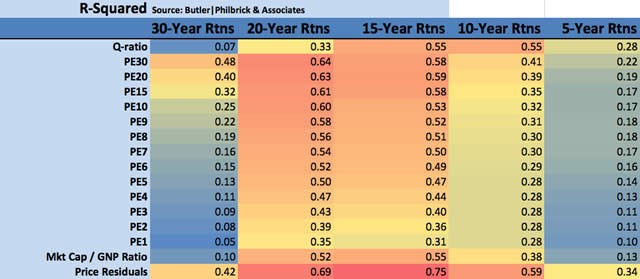
The following matrices show the R-Squared ratio, regression slope, regression intercept, and current predicted forecast returns for each valuation factor. The matrices are heat-mapped so that larger values are reddish, and small or negative values are blue-ish. Note that for the purposes of our regression analysis we have normalized the valuation metrics by using an ordinal ranking system. This approach reduces the impact of large statistical outliers, such as the 1998 – 2000 technology bubble, which have the potential to contaminate our model. As such, the equations defined by the matrices below do not take nominal valuation metrics as inputs, but rather take the ordinal rank of each valuation metric instead. Click on each image for a large version.

Matrix 1. Explanatory power of valuation/future returns relationships

Source: Shiller (2011), DShort.com (2011), Chris Turner (2011), World Exchange Forum (2011), Federal

Reserve (2011), Butler|Philbrick & Associates (2011)

You will note that the R-Squared (top chart), which is a very general measure of the explanatory power of the relationship, is highest for the price residuals, market cap to GNP, PE30 – PE15, and Q-ratio over a 15-year forecast horizon (in that order). The explanatory power of smoothed earnings ratios gets better consistently as we extend the forecast horizon, with peak ratios at the 20 to 30-year range. No factors possess any material explanatory ability at forecast horizons less than 5 years, so we have omitted results for these horizons.

Many analysts quote ‘Trailing 12-Months’ or TTM PE ratios for the market as a tool to assess whether markets are cheap or expensive. If you hear an analyst quoting the market’s PE ratio, odds are they are referring to this TTM number. Our analysis slightly modifies this measure by averaging the PE over the prior 12 months rather than using trailing cumulative earnings through the current month, but this change does not substantially alter the results. As it turns out, TTM average earnings is the least prescriptive of the indicators studied at all horizons, though it does provide the most optimistic forecasts. Perhaps this is why it is so widely quoted by most market strategists. Just remember that these analysts have no proven ability whatsoever in predicting market returns (see here,  here, and here). Further, it can be argued that their firms have a substantial incentive to keep their clients invested in stocks.

Forecasting Expected Returns

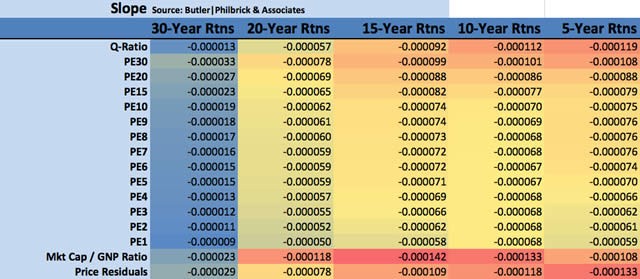
The next matrices provide the slope and intercept coefficients for each regression. We have provided these in order to illustrate how we calculated the values for Matrix 4. below of forecast future returns to stocks.

Matrix 2. Slope of regression line for each valuation factor/time horizon pair.

Source: Shiller (2011), DShort.com (2011), Chris Turner (2011), World Exchange Forum (2011), Federal

Reserve (2011), Butler|Philbrick & Associates (2011)

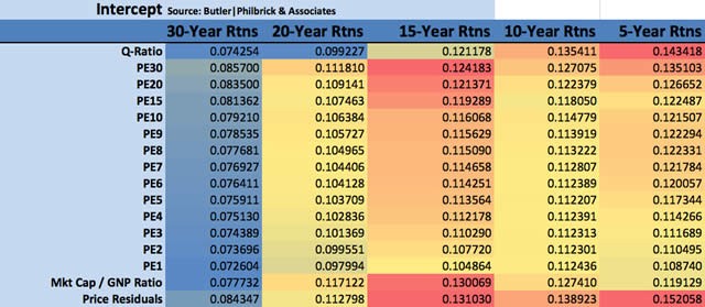
Matrix 3. Intercept of regression line for each valuation factor/time horizon pair.

Source: Shiller (2011), DShort.com (2011), Chris Turner (2011), World Exchange Forum (2011), Federal

Reserve (2011), Butler|Philbrick & Associates (2011)

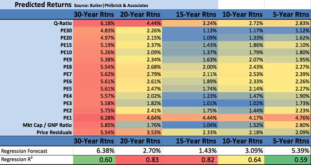
Our final matrix below shows forecast future real returns over each time horizon, as calculated from the slopes and intercepts above, by using the most recent values for each of the 13 earnings series, the Q-Ratio, market cap / GNP, and the return series as inputs. For example, the 15-year return prediction based on the current Q-Ratio can be calculated by multiplying the current ordinal rank of the Q-Ratio (967) by the slope from Matrix 2. at the intersection of ‘Q-Ratio’ and ’15-Year Rtns’ (-0.0000918), and then adding the intercept at the same intersection (0.121178) from Matrix 3. The result is 0.0324, or 3.24%, as you can see in Matrix 4 below at the same intersection (Q-Ratio : 15-Year Rtns). Please click the matrix for a larger version.

Matrix 4. Modeled forecast future returns using current valuations.

Source: Shiller (2011), DShort.com (2011), Chris Turner (2011), World Exchange Forum (2011), Federal

Reserve (2011), Butler|Philbrick & Associates (2011)

At the bottom of Matrix 4. we have calculated the forecast returns over each future horizon based on our best-fit multiple regression from the factors above. We began testing the multiple regression against the Q- ratio, the 15-year Shiller PE, the price regression, and the market cap to GNP as a 4 factor model. However, we discovered that the smoothed PE ratios provide more noise than signal to the regression (that is, these factors were not statistically significant and reduced the F-score), so we narrowed the regression to include just the Q ratio, market cap/GNP, and the real price series over each forecast horizon. We provided the R- squared for each multiple regression at the bottom of each forecast horizon column in Matrix 4.; you can see that at the 15-year forecast horizon, our regression explains 82% of total returns to stocks. Further, the regression is very highly statistically significant, with a p value of effectively zero.

Chart 2. below demonstrates how closely the model tracks actual future 15-year returns. The red line tracks the model’s forecast annualized real total returns over subsequent 15-year periods, while the blue line shows the actual annualized real total returns over the same 15-year horizon.

Chart 2. 15-Year Forecast Returns vs. 15-Year Actual Future Returns

Source: Shiller (2011), DShort.com (2011), Chris Turner (2011), World Exchange Forum (2011), Federal

Reserve (2011), Butler|Philbrick & Associates (2011)

You can see that 15-year ‘Regression Forecast’ expected returns are 1.43% per year, and 10-year returns are forecast to be 3.09% per year using market valuations to September 21, 2011. To be clear, despite the market’s selloff over the last several months, our model still forecasts real total returns to U.S. stocks over the next 15 years of less than 1.5%. Regression analysis also measures the potential deviation from estimates (standard error of coefficients), so we can say there is a 95% chance that returns will be less than 5.4% over the next 15 years. In other words, we are 95% certain that stocks will underperform their long- term average returns over the next 15 years.

Putting the Predictions to the Test

A model is not very interesting or useful unless it actually does a good job of predicting the future. To that end, we tested the model’s predictive capacity at some key turning points in markets over the past century to see how well it forecast future inflation-adjusted total returns.

Table 2. Comparing Long-term average forecasts with model forecasts

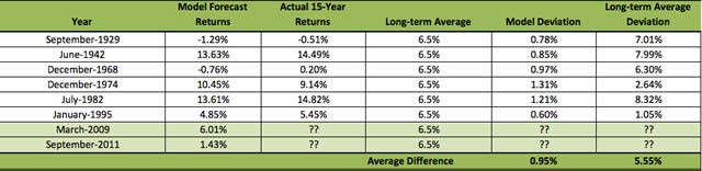
Source: Shiller (2011), DShort.com (2011), Chris Turner (2011), World Exchange Forum (2011), Federal

Reserve (2011), Butler|Philbrick & Associates (2011)

You can see we tested against periods during the Great Depression, the 1970s inflationary bear market, the 1982 bottom, and the middle of the 1990s technology bubble in 1995. The table also shows expected 15- year returns given market valuations at the 2009 bottom, and current levels. These are shaded green because we do not have 15-year future returns from these periods yet. Note real total return forecasts of 6.01% annualized from the bottom of the market in February 2009. This suggests that prices just approached fair value at the market’s bottom, but they were nowhere near the level of cheapness that markets achieved at bottoms in 1932 or 1982. As of the September 21, 2011, expected future returns over the next 15 years are 1.43 percent.

We compared the forecasts from our model with what would be expected from using just the long-term average real returns of 6.5% as a constant forecast, and demonstrated that estimates form long-term average returns yield over 500% more error than estimations from our model over these 15-year forecast horizons (0.95% annualized return error from our model vs 5.55% using the long-term average). Clearly the model offers substantially more insight into future return expectations than simple long-term averages, especially near valuation extremes.

Conclusions

The ‘Regression Forecast’ return predictions along the bottom of Matrix 4. are robust forecasts of future stock returns, as they account for over 100 different cuts of the data, using 3 distinct valuation techniques, and utilize the most explanatory statistical relationships. The models explain up to 82% of future returns based on R-Squared, and are statistically significant at p~0. It is worth noting, however, that even this model has very little explanatory power over horizons less than 6 or 7 years, so almost anything is possible in the short-term. For the next 15 years however, we can say with some confidence that our best estimate of annualized returns is 1.43%, with an optimistic upside estimate of 5.4%.

Investors would do well to heed the results of robust statistical analyses of actual market history, and play to the relative odds. This analysis suggests that markets are currently expensive, and asserts a very high probability of low returns to stocks (and possibly other asset classes) in the future. Remember, any returns earned above the average are necessarily earned at someone else’s expense, so it will likely be necessary to do something radically different than everyone else to capture excess returns going forward.